04. Gradient-based vs. Binary Descriptors
Gradient-based vs. Binary Descriptors
ND313 C03 L03 A08 C34 Intro
Detectors and Descriptors
Before we go into details on how some of the keypoint detectors discussed in the previous section work, let us take a look at the problem ahead of us. Our task is to find corresponding keypoints in a sequence of images that we can use to compute the TTC to a preceding object, e.g. a vehicle. We therefore need a way to robustly assign keypoints to each other based on some measure of similarity. In the literature, a large variety of similarity measures (called descriptors ) have been proposed and in many cases, authors have published both a new method for keypoint detection as well as similarity measure which has been optimized for their type of keypoints.
Let us refine our terminology at this point :
- A keypoint (sometimes also interest point or salient point) detector is an algorithm that chooses points from an image based on a local maximum of a function, such as the "cornerness" metric we saw with the Harris detector.
- A descriptor is a vector of values, which describes the image patch around a keypoint. There are various techniques ranging from comparing raw pixel values to much more sophisticated approaches such as histograms of gradient orientations.
Descriptors help us to assign similar keypoints in different images to each other. As shown in the figure below, a set of keypoints in one frame is assigned keypoints in another frame such that the similarity of their respective descriptors is maximized and (ideally) the keypoints represent the same object in the image. In addition to maximizing similarity, a good descriptor should also be able to minimize the number of mismatches, i.e. avoid assigning keypoints to each other that do not correspond to the same object.
.jpg)
Before we go into details on a powerful class of detector / descriptor combinations (i.e. binary descriptors such as BRISK), let us briefly revisit one of the most famous descriptors of all time - the Scale Invariant Feature Transform. The reason we are doing this is two-fold : First, this method is still relevant and being used in a large number of applications. And second, we need to lay some foundations so that you will be able to better understand and appreciate the contributions of binary descriptors.
HOG Descriptors and SIFT
ND313 Timo Intv 10 Can You Describe SIFT
In the following, we will take a brief look at the family of descriptors based on Histograms of Oriented Gradients (HOG). The basic idea behind HOG is to describe the structure of an object by the distribution its intensity gradients in a local neighborhood. To achieve this, an image is divided into cells in which gradients are computed and collected in a histogram. The set of histogram from all cells is then used as a similarity measure to uniquely identify an image patch or object.
One of the best-known examples of the HOG family is the Scale-Invariant Feature Transform (SIFT), introduced in 1999 by David Lowe. The SIFT method includes both a keypoint detector as well as a descriptor and it follows a five-step process, which is briefly outlined in the following.
- First, keypoints are detected in the image using an approach called „Laplacian-Of-Gaussian (LoG)“, which is based on second-degree intensity derivatives. The LoG is applied to various scale levels of the image and tends to detect blobs instead of corners. In addition to a unique scale level, keypoints are also assigned an orientation based on the intensity gradients in a local neighborhood around the keypoint.
- Second, for every keypoint, its surrounding area is transformed by removing the orientation and thus ensuring a canonical orientation . Also, the size of the area is resized to 16 x 16 pixels, providing a normalized patch.
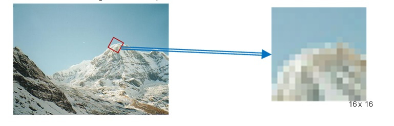
The mountain scenery image material has been taken from the original publication by D. Lowe.
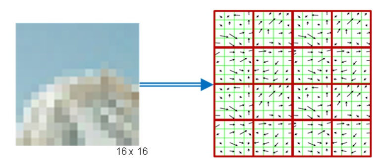
- Third, the orientation and magnitude of each pixel within the normalized patch are computed based on the intensity gradients Ix and Iy.
- Fourth, the normalized patch is divided into a grid of 4 x 4 cells. Within each cell, the orientations of pixels which exceed a threshold on magnitude are collected in a histogram consisting of 8 bins.
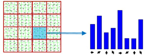
- Last, the 8-bin histograms of all 16 cells are concatenated into a 128-dimensional vector (the descriptor) which is used to uniquely represent the keypoint.
The SIFT detector / descriptor is able to robustly identify objects even among clutter and under partial occlusion. It is invariant to uniform changes in scale, to rotation, to changes in both brightness and contrast and it is even partially invariant to affine distortions.
The downside of SIFT is its low speed, which prevents it from being used in real-time applications on e.g. smartphones. Other members of the HOG family (such as SURF and GLOH), have been optimized for speed. However, they are still too computationally expensive and should not be used in real-time applications. Also, SIFT and SURF are heavily patented, so they can’t be freely used in a commercial context. In order to use SIFT in the OpenCV, you have to
#include <opencv2/xfeatures2d/nonfree.hpp>
, which further emphasizes this issue.
A much faster (and free) alternative to HOG-based methods is the family of binary descriptors, which provide a fast alternative at only slightly worse accuracy and performance. Let us take a look at those in the next section.
Binary Descriptors and BRISK
The problem with HOG-based descriptors is that they are based on computing the intensity gradients, which is a very costly operation. Even though there have been some improvements such as SURF, which uses the integral image instead, these methods do not lend themselves to real-time applications on devices with limited processing capabilities (such as smartphones).
The central idea of binary descriptors is to rely solely on the intensity information (i.e. the image itself) and to encode the information around a keypoint in a string of binary numbers, which can be compared very efficiently in the matching step, when corresponding keypoints are searched. Currently, the most popular binary descriptors are BRIEF, BRISK, ORB, FREAK and KAZE (all available in the OpenCV library).
From a high-level perspective, binary descriptors consist of three major parts:
- A sampling pattern which describes where sample points are located around the location of a keypoint.
- A method for orientation compensation , which removes the influence of rotation of the image patch around a keypoint location.
- A method for sample-pair selection , which generates pairs of sample points which are compared against each other with regard to their intensity values. If the first value is larger than the second, we write a '1' into the binary string, otherwise we write a '0'. After performing this for all point pairs in the sampling pattern, a long binary chain (or ‚string‘) is created (hence the family name of this descriptor class).
In the following, the "Binary Robust Invariant Scalable Keypoints (BRISK)" keypoint detector / descriptor is used as a representative for the binary descriptor family. Proposed in 2011 by Stefan Leutenegger et al., BRISK is a FAST-based detector in combination with a binary descriptor created from intensity comparisons retrieved by dedicated sampling of each keypoint neighborhood.
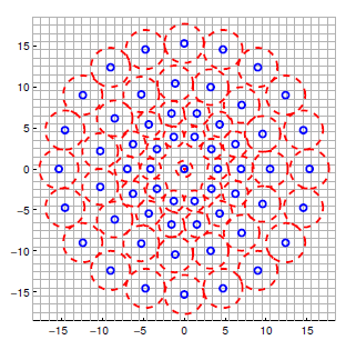
The sampling pattern of BRISK is composed out of a number of sample points (blue), where a concentric ring (red) around each sample point denotes an area where Gaussian smoothing is applied. As opposed to some other binary descriptors such as ORB or BRIEF, the BRISK sampling pattern is fixed. The smoothing is important to avoid aliasing (an effect that causes different signals to become indistinguishable - or aliases of one another - when sampled).
During sample pair selection, the BRISK algorithm differentiates between long- and short-distance pairs. The long-distance pairs (i.e. sample points with a minimal distance between each other on the sample pattern) are used for estimating the orientation of the image patch from intensity gradients, whereas the short-distance pairs are used for the intensity comparisons from which the descriptor string is assembled. Mathematically, the pairs are expressed as follows:
.png)
First, we define the set A of all possible pairings of sample points. Then, we extract the subset L from A for which the euclidean distance is above a pre-defined upper threshold. This set are the long-distance pairs used for orientation estimation. Lastly, we extract those pairs from A whose euclidean distance is below a lower threshold. This set S contains the short-distance pairs for assembling the binary descriptor string.
The following figure shows the two types of distance pairs on the sampling pattern for short pairs (left) and long pairs (right).
 \]](img/new-group-1.jpg)
[based on this [source](based on https://www.cse.unr.edu/~bebis/CS491Y/Lectures/BRISK.pptx ) ]
From the long pairs, the keypoint direction vector \vec{g} is computed as follows:
.png)
First, the gradient strength between two sample points is computed based on the normalized unit vector that gives the direction between both points multiplied with the intensity difference of both points at their respective scales. In (2), the keypoint direction vector \vec{g} is then computed from the sum of all gradient strengths.
Based on \vec{g} , we can use the direction of the sample pattern to rearrange the short-distance pairings and thus ensure rotation invariance. Based on the rotation-invariant short-distance pairings, the final binary descriptor can be constructed as follows:
.png)
After computing the orientation angle of the keypoint from g, we use it to make the short-distance pairings invariant to rotation. Then, the intensity between all pairs in S is compared and used to assemble the binary descriptor we can use for matching.
HOG vs. Binary Exercise
ND313 C03 L03 A09 C34 Outro
In the code at the end of this section, keypoints and descriptors are computed using the BRISK method. The time for both keypoint detection and descriptor computation is printed to the console. For the BRISK detector, the keypoints can be seen in the following figure with the center of a circle denoting its location and the size of the circle reflecting the characteristic scale.
.png)
Given the code in
describe_keypoints.cpp
of the workspace below, add the SIFT detector / descriptor, compute the time for both steps and compare both BRISK and SIFT with regard to processing speed and the number and visual appearance of keypoints.
After building your code with
cmake
and
make
, you can run the code from the virtual desktop using the
describe_keypoints
executable.
Workspace
This section contains either a workspace (it can be a Jupyter Notebook workspace or an online code editor work space, etc.) and it cannot be automatically downloaded to be generated here. Please access the classroom with your account and manually download the workspace to your local machine. Note that for some courses, Udacity upload the workspace files onto https://github.com/udacity , so you may be able to download them there.
Workspace Information:
- Default file path:
- Workspace type: react
- Opened files (when workspace is loaded): n/a
-
userCode:
             export CXX=g++-7


              export CXXFLAGS=-std=c++17
In the next section, we will look at the descriptor part of BRISK in detail.